Samplers comparison
License
rosenbrock_simple
Sun Apr 02 21:13:00 2023
Copyright 2023
Sandro Dias Pinto Vitenti vitenti@uel.br ___ rosenbrock_simple
Copyright (C) 2023 Sandro Dias Pinto Vitenti vitenti@uel.br
numcosmo is free software: you can redistribute it and/or modify it under the terms of the GNU General Public License as published by the Free Software Foundation, either version 3 of the License, or (at your option) any later version.
numcosmo is distributed in the hope that it will be useful, but WITHOUT ANY WARRANTY; without even the implied warranty of MERCHANTABILITY or FITNESS FOR A PARTICULAR PURPOSE. See the GNU General Public License for more details.
You should have received a copy of the GNU General Public License along with this program. If not, see http://www.gnu.org/licenses/.
import sys

from numcosmo_py import Ncm

import matplotlib.pyplot as plt
import numpy as np
import getdist
import getdist.plots

from numcosmo_py.sampling.apes import APES
from numcosmo_py.sampling.catalog import Catalog
from numcosmo_py.plotting.tools import set_rc_params_article

import emcee
import zeus
from pyhmc import hmc
Initialize NumCosmo and sampling parameters
In this notebook, we will compare the performance of four different samplers: APES, Emcee, Zeus and PyHMC. To start, we will use the new Python interface for NumCosmo.
Next, we will define the sampling configuration. Our goal is to generate a total of 600,000 points across all three samplers, with each sampler using 300 walkers except for PyHMC that generates a single chain. This translates to 2000 steps on each sampler to reach our desired sample size. By comparing the performance of these three samplers using the NumCosmo Python interface, we can evaluate their respective capabilities and identify any advantages or limitations for our specific problem.
Ncm.cfg_init()
Ncm.cfg_set_log_handler(lambda msg: sys.stdout.write(msg) and sys.stdout.flush())

ssize = 600000
nwalkers = 300
burin_steps = 500
verbose = False
Probability definition
In the cell below, we will define the unnormalized Rosenbrock distribution, which is known to be a difficult distribution to sample from. The Rosenbrock distribution is often used as a benchmark for testing the performance of sampling algorithms. By using this challenging distribution, we can better understand how well the samplers perform under difficult sampling conditions.
We will generate a single initial sample point with random normal realizations having a mean of zero and a standard deviation of one. This initial point will be used as the starting point for each of the samplers, ensuring that they all start at the same point.
It’s worth noting that this initial sample point is very different from a sample from an actual Rosenbrock distribution. However, this is intentional, as we want to see how each sampler performs under challenging conditions.
def log_prob(x, ivar):
    return -0.5 * (100.0 * (x[1] - x[0] * x[0]) ** 2 + (1.0 - x[0]) ** 2) * 1.0e-1


def log_prob_grad(x, ivar):
    logp = -0.5 * (100.0 * (x[1] - x[0] * x[0]) ** 2 + (1.0 - x[0]) ** 2) * 1.0e-1
    grad = [
        -0.5
        * (100.0 * 2.0 * (x[1] - x[0] * x[0]) * (-2.0 * x[0]) - 2.0 * (1.0 - x[0]))
        * 1.0e-1,
        -0.5 * (100.0 * 2.0 * (x[1] - x[0] * x[0])) * 1.0e-1,
    ]
    return logp, np.array(grad)


ndim, nwalkers = 2, nwalkers
p0 = np.random.randn(nwalkers, ndim)
Running NumComo’s APES
In the cell below, we will run NumCosmo’s APES algorithm using the configuration defined above.
sampler_apes = APES(
    nwalkers=nwalkers, ndim=ndim, model=None, log_prob=log_prob, args=()
)
sampler_apes.run_mcmc(p0, ssize // nwalkers)
mcat_apes = sampler_apes.get_catalog()
mcat_apes.trim(burin_steps)
Running Emcee
In the cell below, we will run the Emcee algorithm with the same initial
point p0 generated previously. We will generate a chain of samples
using Emcee and store the resulting chain in a Catalog object. This
will allow us to apply the same tests to all algorithms and compare
their performance on an even footing.
sampler_emcee = emcee.EnsembleSampler(nwalkers, ndim, log_prob, args=[0])
state_emcee = sampler_emcee.run_mcmc(p0, ssize // nwalkers)
chain_emcee = sampler_emcee.get_chain(flat=True)
log_prob_emcee = sampler_emcee.get_log_prob(flat=True)
mcat_emcee = Catalog(ndim=ndim, nwalkers=nwalkers, run_type="EMCEE")
mcat_emcee.add_points_m2lnp(chain_emcee, -2.0 * log_prob_emcee)
mcat_emcee.trim(burin_steps)
Running Zeus
In the cell below, we will run the Zeus algorithm with the same initial
point p0 generated previously. We will generate a chain of samples
using Zeus and store the resulting chain in a Catalog object. One
difference from Emcee is that Zeus output chains are not interweaved, so
we need to inform the Catalog object of this fact to ensure that
autocorrelation estimates are correct.
sampler_zeus = zeus.EnsembleSampler(nwalkers, ndim, log_prob, args=[0], verbose=verbose)
sampler_zeus.run_mcmc(p0, ssize // nwalkers, progress=False)
chain_zeus = sampler_zeus.get_chain(flat=True)
log_prob_zeus = sampler_zeus.get_log_prob(flat=True)
mcat_zeus = Catalog(ndim=ndim, nwalkers=nwalkers, run_type="ZEUS")
mcat_zeus.add_points_m2lnp(chain_zeus, -2.0 * log_prob_zeus, interweaved=False)
mcat_zeus.trim(burin_steps)
Running pyhmc: Hamiltonian Monte Carlo
In the cell below, we will run the pyhmc algorithm with the same initial
point p0 generated previously, however since pyhmc is not an ensemble
sampler we use only the first point. We will generate a chain of samples
using pyhmc and store the resulting chain in a Catalog object.
Moreover, here we need to remove a longer burn-in period of 1000
samples, since pyhmc is not an ensemble sampler.
chain_pyhmc, log_prob_pyhmc = hmc(
    log_prob_grad,
    x0=np.array(p0[0]),
    args=(np.array([0]),),
    n_samples=ssize,
    return_logp=True,
)
mcat_pyhmc = Catalog(ndim=ndim, nwalkers=1, run_type="PyHMC")
mcat_pyhmc.add_points_m2lnp(chain_pyhmc, -2.0 * log_prob_zeus)
mcat_pyhmc.trim(ssize // 2)
Analyzing results
In the cell below, we will create two arrays containing the true values
for the mean and standard deviation of the Rosenbrock distribution. We
will then call print_status on each catalog to obtain the current
mean, standard deviation, mean standard deviation, and autocorrelation
time τ. Based on the results, we can see that APES has the lowest
autocorrelation time τ for all parameters, being between 50-100 times
smaller than the autocorrelation time obtained by Emcee and Zeus.
This indicates that APES was able to explore the parameter space more efficiently and produce less correlated samples. Additionally, we can see that the mean, standard deviation and mean standard deviation obtained by all samplers are close to the true values of the Rosenbrock distribution. However, it is important to note that the Emcee and Zeus chains may not have fully converged yet, so it is possible that their mean and variance estimates, as well as their autocorrelation times, could improve with further sampling.
sigma = np.sqrt([10.0, 2401 / 10])
mean = np.array([1.0, 11.0])

Ncm.cfg_msg_sepa()
mcat_apes.print_status()
Ncm.cfg_msg_sepa()
mcat_emcee.print_status()
Ncm.cfg_msg_sepa()
mcat_zeus.print_status()
Ncm.cfg_msg_sepa()
mcat_pyhmc.print_status()
#----------------------------------------------------------------------------------
# NcmMSetCatalog: Current mean:   2.0118       1.0021       11.103
# NcmMSetCatalog: Current msd:    0.0079207    0.012742     0.074897
# NcmMSetCatalog: Current sd:     1.9888       3.1781       15.276
# NcmMSetCatalog: Current var:    3.9551       10.1         233.36
# NcmMSetCatalog: Current tau:    7.138        7.234        10.817
#----------------------------------------------------------------------------------
# NcmMSetCatalog: Current mean:   1.5951       0.60027      6.0177
# NcmMSetCatalog: Current msd:    0.021953     0.09409      0.3077
# NcmMSetCatalog: Current sd:     1.6006       2.3792       7.3684
# NcmMSetCatalog: Current var:    2.5621       5.6608       54.294
# NcmMSetCatalog: Current tau:    84.648       703.76       784.71
#----------------------------------------------------------------------------------
# NcmMSetCatalog: Current mean:   1.7673       0.97194      8.5758
# NcmMSetCatalog: Current msd:    0.028349     0.046361     0.30815
# NcmMSetCatalog: Current sd:     1.7064       2.7625       11.019
# NcmMSetCatalog: Current var:    2.912        7.6313       121.41
# NcmMSetCatalog: Current tau:    124.2        126.74       351.94
#----------------------------------------------------------------------------------
# NcmMSetCatalog: Current mean:   1.7126       0.53742      2.8218
# NcmMSetCatalog: Current msd:    0.028136     0.13137      0.45803
# NcmMSetCatalog: Current sd:     2.0903       1.5917       3.3861
# NcmMSetCatalog: Current var:    4.3695       2.5336       11.465
# NcmMSetCatalog: Current tau:    54.353       2043.4       5489.3
Comparing the mean estimates
Below, we compare the mean estimates obtained by each sampler and print the relative error on each estimate. As we can see, APES is the only sampler that is able to recover the true means within 1% - 2% error, while Emcee and Zeus exhibit much larger errors.
print(np.abs(mcat_apes.get_mean() / mean - 1.0))
print(np.abs(mcat_emcee.get_mean() / mean - 1.0))
print(np.abs(mcat_zeus.get_mean() / mean - 1.0))
print(np.abs(mcat_pyhmc.get_mean() / mean - 1.0))
[0.0020966  0.00939155]
[0.39972599 0.45293618]
[0.02806083 0.2203813 ]
[0.46258321 0.74347242]
Comparing the standard deviation estimates
Similar to the previous comparison, we now look at the relative error on the standard deviation estimates. Once again, APES performs the best among the samplers, with estimates within 1% - 4% of the true values.
print(np.abs(np.sqrt(np.diagonal(mcat_apes.get_covar())) / sigma - 1.0))
print(np.abs(np.sqrt(np.diagonal(mcat_emcee.get_covar())) / sigma - 1.0))
print(np.abs(np.sqrt(np.diagonal(mcat_zeus.get_covar())) / sigma - 1.0))
print(np.abs(np.sqrt(np.diagonal(mcat_pyhmc.get_covar())) / sigma - 1.0))
[0.00499343 0.01413589]
[0.24761925 0.52446852]
[0.12642799 0.28888953]
[0.49665275 0.78147664]
Using getdist on the chains
In this next cell, we convert the catalog of MCMC chains for each
algorithm into MCSamples objects using the getdist package. This
allows us to easily plot the joint and marginal posterior distributions
of the parameters using the getdist plotter.
mcs_apes = mcat_apes.get_mcsamples("APES")
mcs_emcee = mcat_emcee.get_mcsamples("EMCEE")
mcs_zeus = mcat_zeus.get_mcsamples("ZEUS")
mcs_pyhmc = mcat_pyhmc.get_mcsamples("PyHMC")
Removed no burn in
Removed no burn in
Removed no burn in
Removed no burn in
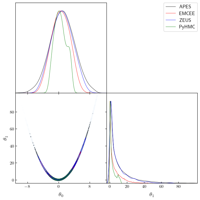
Corner plot
Finally, we create a joint corner plot of the samples using getdist.
We can see that the other samplers (Emcee and Zeus) have more difficulty
in sampling the tails, leading to the 1D marginals being more
concentrated and reporting smaller variance. This is reflected in the
larger relative errors in the mean and standard deviation estimates we
saw earlier.
set_rc_params_article(ncol=2)

g = getdist.plots.get_subplot_plotter(width_inch=plt.rcParams["figure.figsize"][0])
g.settings.linewidth = 0.01
g.triangle_plot([mcs_apes, mcs_emcee, mcs_zeus, mcs_pyhmc], shaded=True)
auto bandwidth for theta_0 very small or failed (h=0.0005832638183669094,N_eff=38411.13458893739). Using fallback (h=0.022408377246589863)
auto bandwidth for theta_1 very small or failed (h=0.0006114885736063465,N_eff=112997.872249284). Using fallback (h=0.003704573608527487)
auto bandwidth for theta_1 very small or failed (h=0.0014299159644314198,N_eff=14883.212703556037). Using fallback (h=0.007191755509401264)
fine_bins_2D not large enough for optimal density: theta_0, theta_1
fine_bins_2D not large enough for optimal density: theta_0, theta_1
fine_bins_2D not large enough for optimal density: theta_0, theta_1